Large-scale Data Processing

To improve database performance and capacity, two options are available:

1. Scale up: buy larger machines
2. Scale out: more machines with parallel execution

Performance metrics:

• Throughput: the number of transactions or queries that can be processed per unit of time

• Response time: the time taken for a transaction or query to be processed

Node: a single machine or server that is part of a larger database cluster. Each node stores a portion of the database's data and can process queries independently or in coordination with other nodes.

Speedup - the improvement in performance or execution time of a task achieved by using multiple nodes in comparison to performing the same task on a single node.

Example

If a task takes 100 seconds to complete on one processor and 25 seconds to complete using four processors, the speedup is:

$$\text{Speedup} = \frac{\text{Time with one processor}}{\text{Time with multiple processors}} = \frac{100}{25} = 4$$

More nodes means more machines with parallel execution, which means more throughput and possibly lower response time.

Speedup is non-linear due to various reaons such as overhead of communication between nodes, coordinating the execution of queries, and execution load not being perfectly equally distributed.

Instead of increasing the number of loads, we can also increase the capacity of existing nodes, enabling the handling of larger loads and more complex operations. This would have no effect on throughput, but allow queries with large data loads to be executed with the same response time.

Parallel Query Evaluation

• Inter-query parallelism: Different queries run in parallel on different nodes

• Intra-query parallelism: A single query is broken down into multiple parts and each part is executed in parallel on different nodes

  • Inter-operator parallelism: Different operators in a query run on different nodes.
  • Intra-operator parallelism: A single operator is broken down into multiple parts and each part is executed in parallel on different nodes

Horizontal Data Partitioning(Sharding)

The tuples in the table are partitioned into chunks according to some partition key, with each table partition is in a different node. The location of each tuple is stored in a key-value table. By allowing data to be distributed across nodes, it improves perfomance and scalability.

Hash Partition

Data is partitioned using a hash function on some attribute X:

• Hash function is a function that takes in an X value and returns a hash value. e.g r.X mod(N) where N is the number of partitions
• Record r goes to chunk i if hash(r.X) mod N = i

Range Partition

Data is partitioned into ranges on some attribute X:

• partition all possible values of attribute X into ranges. e.g X=[1, 2, 3, 4, 5] -> [1-2], [2-3], [3-4], [4-5]
• Record r goes to chunk i if r.X is in the range of chunk i

Example parallel selection

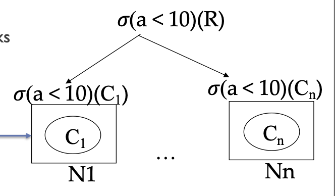
Execution path

1. Push selection to nodes that contain the relevant chunks of data
2. execute the selection locally at each node
3. send result to a coordinating node
4. Assemble result and return to user

Projection and Aggregation operators can also be done locally at each node, howevever in the case of aggregation, there will be different post-processing needed depending on the aggregation function - e.g min of mins

Example parallel join

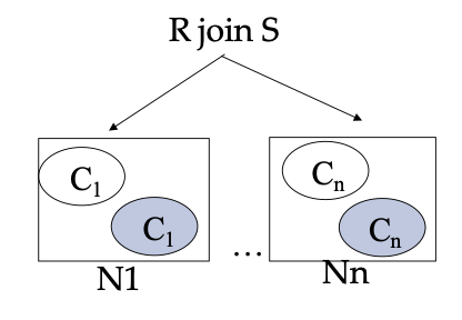
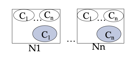
both relations R and S are partitioned into nodes. however since a join requires a cross product, each node will have to perform a cross product with all other nodes. Thus the join can be done as follows:

1. For each node that contains a chunk of the larger relation, copy the chunks of the smaller relation
2. Do the join within each node locally
3. Merge the results

Vertical Data Partitioning

Same idea, except the data is not partitioned by rows(tuples) but by columns, e.g a table with columns A, B, C, and D might be split into two partitions: one with columns A and B, and another with columns C and D.

This type of partitioning is useful for improving performance and managing large datasets by separating frequently accessed columns from those accessed less frequently.

Map-Reduce

A general purpose distributed computing programming model developed by Google. Yahoo devoped open source version Hadoop.

Programming model

Data is distributed across nodes, with each nodes reading records one by one. Each data record is in the format of key-value pairs, where the value is the data and the key is a unique identifier for the data e.g. its hash value.

• Map tasks: Take as input the data records and does some processing/extraction, returning a new set of data records in the format of key-value pairs.
• Reduce tasks: Take as input the key-value pairs and does some processing/aggregation/filtering, returning a new set of data records in the format of key-value pairs.

The inputs and outputs are both key-value pairs so that you can have several passes of mapping and reducing.

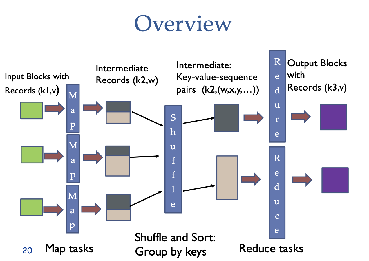
Process flow:

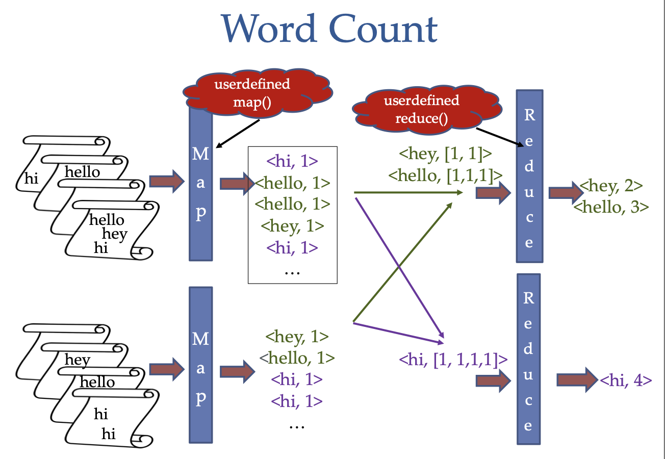
1. Input: The input data is divided into smaller chunks, which are processed independently by multiple map tasks in a completely parallel manner.

2. Map Phase: Each map task processes a chunk of data and produces key-value pairs as output.

3. Shuffling: The system then collects all the keys and values that share the same key from all lists and groups them together, creating one group per key.

4. Reduce Phase: Each group is processed by a reduce task, which takes a key and its corresponding list of values and combines those values into a smaller set of values or a single value.

5. Output: The output from the reduce tasks is the final result of the MapReduce job.

Internal Implementation

• There is one coordinator node that orchestrates the MapReduce job.
• The coordinator node partitions the file into m partitions and assigns workers (server processes) for all m map task and all r reduce task.
• The coordinator node collects the map outputs and distributes them to the reduce tasks
• The coordinator node collects the reduce outputs and combines them to produce the final result
• failures are detected by the coordinator, which can restart the failed tasks

Example Map-Reduce task: Word Count

• Input: Document Set DS(K,documenttext)
• Output: For each word w occuring at least once, indicate the number of occurrences of w in DS.

Map step:

The system spits the input data into m user defined partitions. the map function is executed locally on each partition and then the results are combined and given as input to the shuffle step.

1. Input: A text document
2. Map: Split the document into words
3. Output: A list of words and their counts

WordCountMap():
for each input key/value pair(k,documenttext)
    for each word w of dtext
        output key-value pair (w,1)

Shuffle step: The system then sorts the outputs by their key and groups all key-value pairs with the same key (k,v1), (k,v2), (k,v3)... into (k,(v1,v2,v3...))

Reduce step:

After shuffling and sorting, the system partitions the outputs into r partitions, and the reduce taks is run on each partition locally. The output of the reduce tasks are then combined to produce the final result. The value of r is user defined.

1. Input: A list of words and their counts
2. Reduce: Sum the counts of each word
3. Output: A list of words and their total counts

wordCountReduce():
for each input key/value-list pair (k,(v1,v2,v3...))
    output (k,sum(v1,v2,v3...))

Selection with Map/reduce

Assume a relation R(A,B,C,D) on which we want to do a selection with condition c

Then the map function is as follows:

selectionMap():
for each input key/value pair(k,tuple)
    if c(tuple) is true
        output key-value pair (k,tuple)

and the Reduce value would simply forward the output with no changes, i.e. returns the identity

selectionReduce():
for each input key/value-list pair(k,tuples)
    output key-value pair (k,tuples)

Join with Map/reduce

Assume a natural join R(A,B,C) and Q(C,D,E) Since C is the common attribute,we join the two relations on C.

The map function is as follows:

joinMap():
for each input key/value pair(a(b,c)) of R: // key=a because it is the primary key
    output key-value pair (c,(R(a,b)))

for each input key/value pair(c(d,e)) of Q:
    output key-value pair (c,(Q(d,e)))

Since the tuples are currently in different relations, they cannot be compared directly. Thus the map function is responsible for grouping the tuples by their key (c) and then the reduce function can combine the tuples into a single tuple.

Sort and Shuffle step: The system then sorts the outputs by their key and groups all key-value pairs with the same key into (c,(R(a1,b1),R(a2,b2)...,Q(d1,e1),Q(d2,e2)...))

Reduce step:

produce all combinations of (c,(ai,bi,dj,ej)):

for each tuple (c,(R(a1,b1),R(a2,b2)...,Q(d1,e1),Q(d2,e2)...)):
    Rtable = empty
    Qtable = empty
    for each  (R,(ai,bi)) or (Q,(dj,ej)) in value list:
        if from R, add (ai,bi) to Rtable
        if from Q, add (dj,ej) to Qtable

    for value1 in Rtable:
        for value2 in Qtable:
            output key-value pair (c,(v1,v2)) // i.e (c,(ai,bi,dj,ej))